Forces

Before we talk about internal forces, let’s quickly just talk about what a force is. In the most simplest terms, it’s a push or pull exerted on an object from its interaction with another object. You may have heard of Newton’s Laws of Motions. These 3 laws give a relationship between objects and forces.

Law #1: An object stays at rest or in constant motion unless acted upon by an external force.

Law #2: F = ma (Force = mass * acceleration) (acceleration is change in velocity)

Law #3: For every action, there’s an equal and opposite reaction.

Free Body Diagrams

Let’s also quickly review free body diagrams. A free body diagram is used to look at what forces are acting on something.

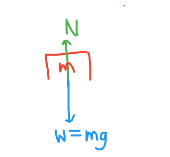
In the image above, first there’s always a weight force pointing downwards from the object. Since it’s sitting on a surface, there’s a normal force pushing up. A normal force is one that’s normal (perpendicular) to the surface. The object is stationary, so that means the object is at equilibrium and the normal and weight forces are equivalent to each other.

Internal Forces

Within a beam, there are 3 forces: Axial Force (P), Shear Force (V) and Bending Moment (M). Let’s talk about each one of these in detail.

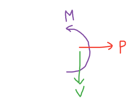
Axial Force (P)

First is the Axial Force (P). From the name, you could probably assume that it’s the force that pushes “sideways”. In other words, it’s the force that acts along the longitudinal axis and it either causes Tension (stretching), or compression (squashing).

Shear Force (V)

Second is the Shear Force (V). This one acts perpendicular to the beam’s axis. It is caused by external forces and the reactions at the supports.

Bending Moment (M)

Lastly is the Bending Moment (M). To begin, the general definition of “moment” is force created by rotation. Bending moment in particular is the internal moment induced by external forces.

In the diagram above, we did a cut that looks at the left side of the beam. If we did a cut that looks at the right side of the beam, all the orientations of the internal forces/moments would be reversed. For example, Axial Force will go towards the left, Shear Force upwards, and Bending moment will be clockwise.

Problem Solving Methods

Whenever we want to find the internal forces in a beam, one way is to do equilibrium of the whole beam, make a “cut” in the beam, analyze all the forces present, create a FBD and solve for the unknowns. This way is pretty straight forward.

Another way is through integrals. We began by taking equilibrium of the whole beam, and then we set up our integrals. These integrals are: \(V_{1} = V_{A} - \int_{0}^{x} W(x) \,dx\) where \(W\) is the distributed force (0 if there are none) and \(V_{A}\) is any external force present at the beginning of the section. The second integral is: \(M_{1} = M_{A} + \int_{0}^{x} V_{1} \,dx\) where \(M_{A}\) is any external moment present at the beginning of the section. We are finding the Shear Force (V) and the Bending Moment (M) here. Usually, we get equations and from there we can graph it to see how the internal forces act through the beam over time.

Example

It’s hard to still understand it through just reading it, so I will do a super simple example. I’m not going to do method 1 since it’s pretty straightforward (yet time consuming sometimes), and method 2 is the much easier and better method.

Method 2

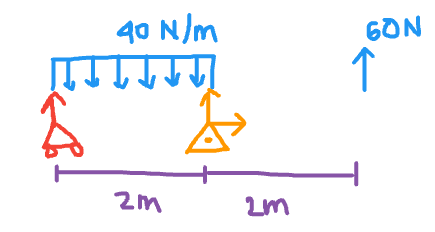
First, let us solve for the distributed force

\(40 \frac{N}{m} \cdot 2m = 80 N\).

We are just taking the area to get the distributed force. Next, the location of the force will be in the center since it’s a rectangle, so at 1m.

There is also an Ay force at the roller support on the far left, and Bx, By forces on the pin support in the middle.

Let’s now take equilibrium (summing up all the forces and setting it equal to 0 since this is a static problem):

\(F_{x}\) Equilibrium: \(\sum_{}^{} F_{x} = B_{x} = 0\)

\(F_{y}\) Equilibrium: \(\sum_{}^{} F_{y} = A_{y} + B_{y} - 80 + 60 = 0\)

\(M_{B}\) Equilibrium: \(\sum_{}^{} M_{B} = -A_{y}(2) + (80)(1) + (60)(2) = 0 \rightarrow A_{y} = 100 N, B_{y} = -80 N\)

Next step is to section off the beam to take the integrals. The logical step would to make \(0 \leq x<2\) Section 1, and \(2 \leq x<4\) Section 2 since the distributed force ends at 2 m.

Now for our integrals. Let’s first find the equations for section 1:

\[V_{1} = V_{A} - \int_{0}^{x} W(x) \,dx\]

First, our \(V_{A}\) will be \(A_{y} = 100 N\), as that’s the external force present at the beginning of the section. Next, \(W(x)\) is the equation of the disributed force. Since it’s just a straight line, it’s just \(y = 40\). If you want, you can even find the slope using points (0,40) and (2,40), giving you a slope of 0 and then plugging it into point-slope form equation, resulting in \(y = 40\). Our bounds are 0 to x, as the section starts at 0m, and we are cutting it to an arbritary ‘x’ m as we want the general equation for the shear force, not the exact shear force at the location.

\[V_{1} = 100 - \int_{0}^{x} 40 \,dx \rightarrow V_{1} = 100 - 40x\]

\[M_{1} = M_{A} + \int_{0}^{x} V(x) \,dx\]

There is no external moment present at the beginning of this section, so our \(M_A\) is just 0. For \(V(x)\), we just plug in the \(V(x)\) we found previously.

\[M_{1} = 0 + \int_{0}^{x} 100 - 40x \,dx \rightarrow M_{1} = 100x - 20x^{2}\]

Now, let’s do section 2, which is from \(2 \leq x < 4\).

\[V_{2} = V_{x=2} + V_{A} - \int_{0}^{x} W(x) \,dx\]

First, our \(V_{A}\) will be \(B_{y} = -80 N\), as that’s the external force present at the beginning of the section. We also need to find the Shear Force at x=2m with our \(V_1\) equation to take into account the shear force at 2m, since our previous integral did not. Next, \(W(x)\) is the equation of the disributed force. Since there is no distributed force from \(2 \leq x < 4\), \(W(x) = 0\). Our bounds are 2 to x, as the section starts at 2m, and we are cutting it to an arbritary ‘x’ m as we want the general equation for the shear force, not the exact shear force at the location.

\[V_{2} = 20 + (-80) - \int_{2}^{x} 0 \,dx \rightarrow V_{2} = -60\]

\[M_{2} = M_{x=2} + M_{A} + \int_{2}^{x} V(x) \,dx\]

There is no external moment present at the beginning of this section, so our \(M_A\) is just 0. We also need to find the Bending Moment at x=2m with our \(M_1\) equation to take into account the bending moment at 2m, since our previous integral did not. For \(V(x)\), we just plug in the \(V(x)\) we found previously.

\[M_{2} = 120 + 0 + \int_{2}^{x} -60 \,dx \rightarrow M_{2} = 240 - 60x\]

We are done finding the equations of the shear force and bending moment for the 2 sections! Now, we can graph it to see how it looks like.

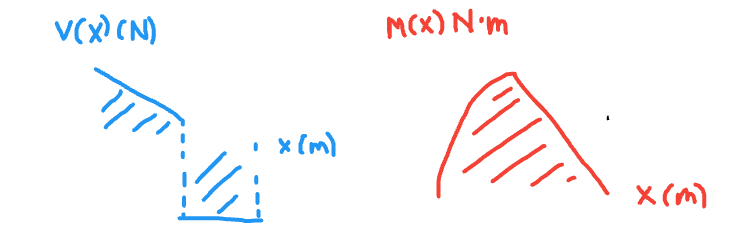
And that’s it! Hopefully this made sorta sense, or at least was interesting to read. Thanks for reading everyone! Please let me know your thoughts :)

Differential Equations are equations that relate some unknown function with its derivatives (rates of change). Usually they are used to model something that’s dynamic, like population growth or circuit behavior.

That’s where the Laplace transform comes in. It can take a function of time, often complicated with many derivatives, and transform it into a new function of variable ‘s’. Now, derivatives become multiplication and solving these differential equations is just like a simple algebraic equation.

Fourier Transform

You may have heard of the Fourier Transform. If you haven’t, it basically decomposes a signal into it’s individual frequency components, in the form of \(e^{j\omega t}\).

The thing is with the Fourier Transform is that it can only work for signals that don’t grow over time - aka it doesn’t really work with unstable/exponential signals.

But the Laplace Transform works for any signal, as it allows it to decay/grow and even oscillate. Instead of \(e^{j\omega t}\), it’s just \(e^{st}\) where s is a complex number.

\[s = \sigma + j\omega\]

where \(\sigma\) is the real part that controls growth/decay and \(j\omega\) is the imaginary part that controls the oscillation frequency

You could say the Fourier Fransform is actually a special case of the Laplace Transform, as it’s when \(\sigma = 0\) and so \(s = j\omega\) is the Fourier transform.

Laplace Transform Definition

Specifically, the Laplace Transform is defined as below:

\[F(s) = \mathcal{L}(f(t)) = \int_{0}^{\infty} f(t) \cdot e^{-st} \,dt\]

First, it’s important that this is right-sided. As in it only looks at values that are positive and to the right of 0. This integral takes EVERY value of the signal f(t) from t=0 to infinity and makes it ONE expression: F(s). The inverse transform also exists, where we go from F(s) to f(t). Since the inverse exists, no information is destroyed and we can easily go back and forth between the two domains.

Laplace Transforms & Differential Equations

Earlier, I said that the Laplace Transform makes solving differential equations much easier. We can now see why as we are just switching it from the time domain to the Laplace domain (where it’s now simple multiplication).

\[\mathcal{L}(f'(t)) = s \cdot F(s) - f(0)\] \[\mathcal{L}(f''(t)) = s^{2} \cdot F(s) - s \cdot f(0) - f'(0)\]

We can keep going until the nth derivative. In the Laplace domain, a 2nd order differential equation would just become a quadratic in s. From there we can solve for F(s), and use a Laplace table to get the inverse, giving us f(t).

Transfer Function H(s)

Another very important characteristic of the Laplace Transform is H(s), or the Transfer Function.

\[H(s) = Y(s) / X(s)\]

The “poles” of H(s) are the values of when the denominator would go to 0. For example, if we had \(\frac{1}{s+2}\), the pole would be s = -2, as then the denominator becomes 0 and it blows up. The location of the poles in the complex s-plane tell us a lot about what will happen to the function. H(s) is also the Laplace transform of h(t), or the impulse response!

In this above image, the green pole at 0 gives us pure decay (\(e^{-at}\)). The 2 other green poles give us damped oscillations (\(e^{-at}sin(\omega t)\)). The red pole at 0 gives us pure growth ((\(e^{at}\))). The 2 other red poles give us growing oscillations (\(e^{at}sin(\omega t)\)). Lastly, the 2 yellow poles on the Im axis are sustained oscillations (\(sin(\omega t)\)). The poles on the left are decaying, so they are stable, while the ones on the right are growing, so they are unstable. Now you could see the connection between the Impulse response h(t) and it’s Laplace Transform, the Transfer Function, H(s). We can see how a system behaves over time through these functions.

Conclusion

Because of these properties, engineers really like using Laplace transforms. By choosing where we set the poles, we are entirely changing the system’s behavior. Instead of modifying the differential equations directly, we can ask “Where should I put the poles so I get the response I want?” And so, all we do is change how we look at something, and make the whole process a whole lot easier for us.

Thanks for reading everyone! I hope you found this topic as interesting as I did. Please let me know your thoughts :)

What is an impulse response? I would like to think of it as a system’s blueprint. All you do is give the system a short burst of energy, a very quick poke, and how the system responds to it is the impulse response. This singular response will tell you how the system would respond to ANYTHING.

Impulse Signal

To get the impulse response, we need to give it some input. This input is what we call the impulse signal or the IMPULSE. In math, we call it the Dirac Delta function, written as \(\delta(t)\). The Dirac Delta is defined as:

\(\delta(t)\) = 0 for all t \(\neq\) 0 and \(\int_{-\infty}^{\infty} \delta(t) \,dt = 1\)

It can be of any width or length (as long as the area is 1), but I like to think of it using the above representation. Physically, the perfect impulse is not possible, but we can come very close to it. There are many practical approximations that work great for most real systems.

Impulse Response h(t)

When you feed a Dirac Delta into a LTI (Linear Time Invarient) system, you get an impulse response output h(t).

system input: \(x(t) = \delta(t)\)

system output: \(y(t) = h(t)\)

Linearity & Time Invarience

It’s very important to note that the system is LTI. Now what does LTI mean exactly? First for linearity. If we have ‘input 1’ and ‘input 2’ of the system, they produce ‘output 1’ and ‘ouput 2’. A linear system would be one that follows the rule that the outputs summed equals the output we get when we put in an input that’s the inputs summed. Aka: y1 + y2 = (x1 + x2). Next for time invarience. Let’s say you flip a switch, and the lightbulb turns blue. You come back a few minutes later, and flip the switch again. It still lights up blue. This means it’s time invarient, as the output (the lightbulb’s color), doesn’t vary with time. Even if you turned on the lightbulb a 10 years from now, it’ll still turn blue.

These properties are so important because it says that any input could be decomposed into individual impulses, and all those impulses added up give the output.

In fact, we can give this an exact value using an integral:

\[x(t) = \int_{}^{} x(\tau) \delta(t-\tau) \,d\tau\]

Convolution

We now apply it to an LTI system. Since it’s linear, each scaled impulse produces a scaled impulse response at the output. Since it’s time invarient, the impulse response to a delayed impulse is just a delayed h(t):

\[y(t) = \int_{}^{} x(\tau) h(t-\tau) \,d\tau\] \[y(t) = x(t) * h(t)\]

The second line is a very important concept called Convolution. If we know h(t), we can find the output for any input forever! It looks something like this:

Stability

Other than predicting outputs, the impulse response can also tell us if a system is stable or unstable. What do we mean by this? We can define a stable system as BIBO stable, as in Bounded Input and Bounded Output. Basically, if the impulse signal eventually decays to 0, the system is stable. But, if it grows or oscillates without ever dying out, it is unstable (bounded inputs producing unbounded outputs). We can see what happens to the overall system just by looking at the impulse response over time.

In real life, we can see many examples of unstable impulse responses. For example, a bridge that sways wider for every gust of wind, eventually leading to failure.

Conclusion

The impulse response is truly so interesting as it takes advantage of very basic and simple characteristics of linear systems. That is, they can’t create new frequencies and they don’t interact with themselves in unpredictable ways across time. To understand a system, we don’t need to set a thousand conditions and study how it reacts to each one of them. We just need to do it once and see what happens.

Thanks for reading everyone! I hope you found this topic as interesting as I did. Please let me know your thoughts :)

Chemistry (CHEM 20B)

This week, I had my 2nd chem midterm on Friday (2/27). It covered concepts from entropy to acid-base calculations. Below is a summary from my Midterm 2 concepts quizlet.

Entropy

Entropy is the possibilities of position. The entropy of gas is higher than liquid than solid since there’s more positions possible. If \(\Delta\)S > 0: more possibilites (spontaneous). If \(\Delta\)S < 0: less possibilities.

Gibbs Free Energy

This the measure of reversible work done at constant temperature and pressure.

• \(\Delta\)G = \(\Delta\)H - T \(\Delta\)S
• \(\Delta\)G > 0, \(\Delta\)S < 0, K < 0(not spontaneous)
• \(\Delta\)G < 0, \(\Delta\)S > 0, K > 1(spontanous)
• \(\Delta\)G = 0 (reversible)

Reaction Quotient Q

• Q < K: shifts right, reactants turn into products (endothermic)
• Q > K: shifts left, products turn into reactants (exothermic)

Acid-Base

• Acid: accepts lone pair, H donator
• Base: donates lone pair, H acceptor
• Conjugate Acid: Base after accepting H
• Conjugate Base: Acid after donating H

Reactions with Acid-Base

• strong acid + strong base: H3O+ + OH- -> 2H20
• strong acid + weak base: H3O+ + B -> HB + H2O
• weak acid + strong base: HA + OH- -> A + H2O

Statics (MAE 101)

I also had a statics quiz today (3/2), so I did a lot of statics studying throughout the week. The professor taught 3 chapters over the course of 3 lectures, so I didn’t really get the material and spent my whole weekend trying to learn it. I think I got an A on the quiz today so I am very glad the studying paid off.

Chp. 14 (Internal Forces & Moments in Beams)

If we have a beam, we could cut the beam at a section to determine the internal forces & moments. These are V (shear force), P (axial force), and M (moment). To determine these internal forces, we must first draw a FBD of the whole beam with all the reactions and solve for them using equilibrium. Afterwards, we cut the beam to determine V, P and M through force balance/equilibrium again.

Another (easier) way to find V, P and M is through the differential method, where \(V = -\frac{dW}{dx}\) and \(M = \frac{dV}{dx}\). In this method, we begin by drawing a FBD and using equilibrium/force balance to solve for the reactions. Then, we can section off the beam. For example, let’s say we have a beam 4 meters long, and in the first half of the bar, there is a distributed force W. We could separate the bar into 2 sections, the half section (\(0 \leq x < 2\) ) with the distributed force, and the other half section (\(2 \leq x < 4\)).

For V1, we would have \(V_{1} = V_{A} - \int_{0}^{x} W(x) \,dx\) where VA is any external (vertical) reaction present at the beginning of the section. \(M_{1} = M_{A} + \int_{0}^{x} V(x) \,dx\), where MA is any external couple present at the beginning of the section. The results will give us V1(x) and M1(x).

For V2, we would have \(V_{2} = V_{A} + V_{x=2} - \int_{0}^{x} W(x) \,dx\), where VA is any external (vertical) reaction present at the beginning of the section and we add that to \(V1_{x=2}\). Similarly, \(M_{2} = M_{A} + M_{x=2} + \int_{2}^{x} V(x) \,dx\) where MA is any external moment present at the beginning of the section.

Chp. 9 (Stress and Strain)

These chapter took me a while to understand the concepts and problems. In short, stress is the amount of force over a specific area. Normal stress is that normal to the plane, while shear stress is that tangential to the plane. We can get normal stress using \(\sigma = \frac{P}{A}\) where P is the axial force and A is the cross-sectional area. The problem solving strategy is drawing an FBD and solving for P. After we get P, we want to draw another FBD right at the plane cut P (different P than axial force), and drawing the stress reactions. We do another force balance here to solve for the normal and shear stresses.

Strain would be how much it’s stretched or shortened when a force is applied. Usually, in these problems, we look for the length by which it changes. The prroblem solving strategy is pretty similar to before, in regards to drawing an FBD and getting P. Here, we have the change in length to be \(\delta = \varepsilon \cdot L\) where \(\varepsilon\) is the strain and L be the original length. Another way it’s commonly written is \(\varepsilon = \frac{dL' - dL}{dL}\) where dL’ is the final length and dL is the original length.

Chp. 10 (Axial loaded bars)

Here, we combine the concepts from chapter 9. The problem solving strategy is pretty much writing down all your knowns and trying to connect the equations in a way to get what you’re solving for. One thing I struggled with here, was the comptability equation when having statically indeterminate problems. This type of problem means that there are more unknowns than number of equations. Thus, we have to use the comptability equation involving \(\delta\). To make it easier to see this, let me write down all the equations we now have. \(\delta = \varepsilon \cdot L\), \(\sigma = E \cdot \varepsilon = \frac{P}{A}\), \(\delta = \frac{PL}{EA}\)

In particular, we use the last definition of \(\delta\) for the compatability equation. If we have it so the bars are side-by-side, it is \(\delta_{1} = \delta_{2}\). If it’s end-to-end, it is \(\delta_{1} + \delta_{2}\). For side-by-side, the bars are sandwiched by top and bottom plates, so they must be squished or stretched by the same amount. For end-to-end, their total change has to be 0 to fit in the space. If one bar is squished, the other bar must stretch.

Conclusion

That’s pretty much it for this week’s learning writeup. It’s already pretty long, so I’m gonna keep it to just classes. I didn’t really do any Chem 20L or ECE 102 studying since I had exams for these classes coming up, but this week I’m gonna do a lot more studying for them.