If you’ve taken Calculus II, you’ve probably came across differential equations, learning methods like integrating factor to solve them. Then in Differential Equations, you start learning about these equations more indepth and some more advanced methods, like variation of parameters and method of undetermined coeffecients. But, these methods at the end of the day are very long and tedious.
Differential Equations are equations that relate some unknown function with its derivatives (rates of change). Usually they are used to model something that’s dynamic, like population growth or circuit behavior.
That’s where the Laplace transform comes in. It can take a function of time, often complicated with many derivatives, and transform it into a new function of variable ‘s’. Now, derivatives become multiplication and solving these differential equations is just like a simple algebraic equation.
You may have heard of the Fourier Transform. If you haven’t, it basically decomposes a signal into it’s individual frequency components, in the form of \(e^{j\omega t}\).
The thing is with the Fourier Transform is that it can only work for signals that don’t grow over time - aka it doesn’t really work with unstable/exponential signals.
But the Laplace Transform works for any signal, as it allows it to decay/grow and even oscillate. Instead of \(e^{j\omega t}\), it’s just \(e^{st}\) where s is a complex number.
\[s = \sigma + j\omega\]
where \(\sigma\) is the real part that controls growth/decay and \(j\omega\) is the imaginary part that controls the oscillation frequency
You could say the Fourier Fransform is actually a special case of the Laplace Transform, as it’s when \(\sigma = 0\) and so \(s = j\omega\) is the Fourier transform.
Specifically, the Laplace Transform is defined as below:
\[F(s) = \mathcal{L}(f(t)) = \int_{0}^{\infty} f(t) \cdot e^{-st} \,dt\]
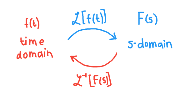
First, it’s important that this is right-sided. As in it only looks at values that are positive and to the right of 0. This integral takes EVERY value of the signal f(t) from t=0 to infinity and makes it ONE expression: F(s). The inverse transform also exists, where we go from F(s) to f(t). Since the inverse exists, no information is destroyed and we can easily go back and forth between the two domains.
Earlier, I said that the Laplace Transform makes solving differential equations much easier. We can now see why as we are just switching it from the time domain to the Laplace domain (where it’s now simple multiplication).
\[\mathcal{L}(f'(t)) = s \cdot F(s) - f(0)\]
\[\mathcal{L}(f''(t)) = s^{2} \cdot F(s) - s \cdot f(0) - f'(0)\]
We can keep going until the nth derivative. In the Laplace domain, a 2nd order differential equation would just become a quadratic in s. From there we can solve for F(s), and use a Laplace table to get the inverse, giving us f(t).
Transfer Function H(s)
Another very important characteristic of the Laplace Transform is H(s), or the Transfer Function.
\[H(s) = Y(s) / X(s)\]
The “poles” of H(s) are the values of when the denominator would go to 0. For example, if we had \(\frac{1}{s+2}\), the pole would be s = -2, as then the denominator becomes 0 and it blows up. The location of the poles in the complex s-plane tell us a lot about what will happen to the function. H(s) is also the Laplace transform of h(t), or the impulse response!
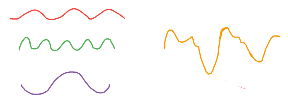
In this above image, the green pole at 0 gives us pure decay (\(e^{-at}\)). The 2 other green poles give us damped oscillations (\(e^{-at}sin(\omega t)\)). The red pole at 0 gives us pure growth ((\(e^{at}\))). The 2 other red poles give us growing oscillations (\(e^{at}sin(\omega t)\)). Lastly, the 2 yellow poles on the Im axis are sustained oscillations (\(sin(\omega t)\)). The poles on the left are decaying, so they are stable, while the ones on the right are growing, so they are unstable. Now you could see the connection between the Impulse response h(t) and it’s Laplace Transform, the Transfer Function, H(s). We can see how a system behaves over time through these functions.
Conclusion
Because of these properties, engineers really like using Laplace transforms. By choosing where we set the poles, we are entirely changing the system’s behavior. Instead of modifying the differential equations directly, we can ask “Where should I put the poles so I get the response I want?” And so, all we do is change how we look at something, and make the whole process a whole lot easier for us.
Thanks for reading everyone! I hope you found this topic as interesting as I did. Please let me know your thoughts :)